Examine outputs

The outputs of a metabarcoding workflow and their basic reading are described in the outputs section of “What is a metabarcoding workflow?”.

In this section, we will examine the outputs of a metabarcoding workflow in relation to user collected environmental metadata to inspect basic patterns of species (metabarcoding features) richness and composition across different environments.

Here, we illustrate the calculation of species (OTU) richness and composition using the metabarcoding outputs from the BGE case study of high mountain systems dataset, restricted here to samples from Norway, as an example. The data are Malaise trap samples collected weekly in 2023 over 20 weeks across 5 altitudes.

We examine:

1. Was sequencing depth sufficient?

2. OTU richness patterns across sampled altitudinal gradient and sampling season.

---

Input data

1. OTU table

2. Sample metadata

example of an OTU table

	sample1	sample2	sample3	sample4	…
OTU_01	579	0	0	0	…
OTU_02	405	345	449	430	…
OTU_03	0	0	231	69	…
OTU_04	0	62	345	0	…

sample metadata

	site	altitude_(m)
sample1	site_01	500
sample2	site_01	500
sample3	site_02	1000
sample4	site_02	1200

Load data

#!/usr/bin/Rscript

# Working directory and results directory paths
wd = "path/to/your/working/directory"
results = file.path(wd, "results")

# OTU table
OTU.table = file.path(wd, "OTU_table.csv")

# Sample metadata
sampleMetadata = file.path(wd, "metadata.csv")

---

Sequencing depth

Sequencing depth is the total number of sequences in a sample. Although the amplicon library is pooled in equimolar concentrations prior to sequencing, there can be still considerable variation in sequencing depth between samples. If so, then for the statistical analyses, it is important to account for this variation.

One way to account for this variation is to normalise sequencing depth to a common value, which can be achieved through rarefaction analysis.

Another way to account for this variation is to use sequencing depth per sample as a covariate in the statistical analyses. By including sequence counts per sample as a predictor, differences in species richness or composition are evaluated after statistically adjusting for variation in sequencing depth.

Note

With the bioinformatic processing (and post-processing steps), we are trying to remove noise from the sequencing data, but this inherently may filter out some true (low abundance) taxa. Therefore, rarfaction analyses after the bioinformatic processing tries to answer the question: “was sequencing depth sufficient to capture the taxa that pass our quality filters?”, not “was sequencing depth sufficient to capture all true taxa in the sample”.

Here, we are examining if the sequencing depth per samples has been sufficient, i.e., do the OTU accumulation curves flatten out (reach the asymptote)?

Sequencing depth per sample

#!/usr/bin/Rscript

# Compute rarefaction curves for each sample
set.seed(1)
library(vegan)
rarecurve_data = rarecurve(
  t(OTU_table),          # transpose so samples are rows
  step  = 5000,          # step size (seqs) in rarefaction curves
  col   = "steelblue",
  label = FALSE
)

# Convert the list returned by rarecurve() into a tidy data frame
library(purrr)
library(dplyr)
library(tidyr)

rarecurve_data_to_ggplot =
  map_dfr(rarecurve_data, bind_rows) %>%
  bind_cols(Group = colnames(OTU_table), .) %>%
  tidyr::pivot_longer(-Group) %>%
  tidyr::drop_na() %>%
  mutate(
    n_seqs = as.numeric(stringr::str_replace(name, "N", ""))
  ) %>%
  select(-name)

# Plot rarefaction curves (richness vs sequences) for all samples
p_rarefaction =
  ggplot(data = rarecurve_data_to_ggplot,
      aes(x = n_seqs, y = value, group = Group)) +
  geom_line(alpha = 0.6, color = "steelblue")  +
  theme_minimal() +
  labs(x = "Number of sequences",
      y = "Number of OTUs",
      title = "Rarefaction curves per sample") +
  theme(
    legend.text  = element_text(size = 12),
    legend.title = element_text(size = 14),
    axis.text    = element_text(size = 11),
    axis.title   = element_text(size = 12),
    plot.title   = element_text(size = 16)
  )

# Save plot
ggsave(
  filename = file.path(results, "rarefaction_curves.png"),
  plot = p_rarefaction,
  width = 8, height = 6, dpi = 300)

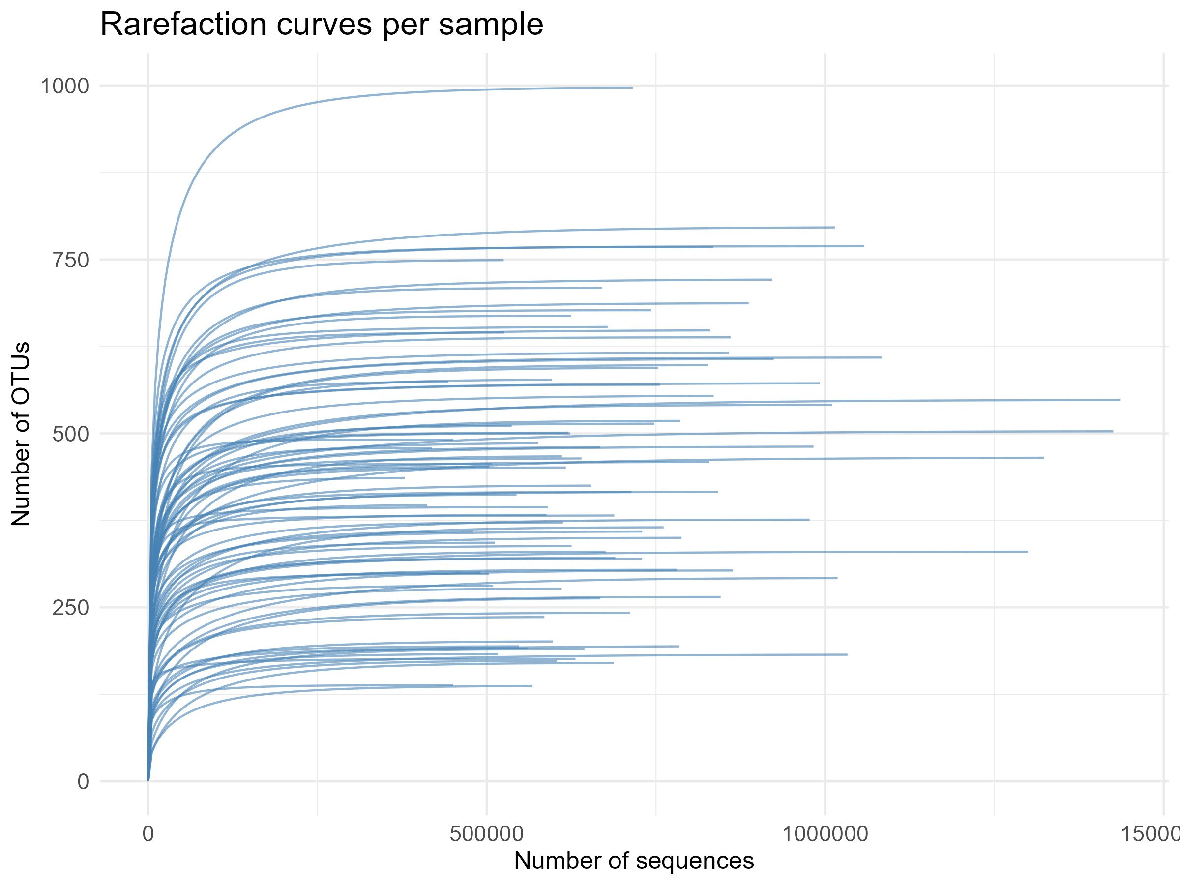
The resulting plot shows the OTU accumulation curves for each sample. Most curves rise steeply at low read numbers and then level off, indicating that additional sequencing yields few (or no) new OTUs and that sequencing depth is generally sufficient for capturing the diversity in these samples.

Now, let’s confirm this by calculating the slope of the rarefaction curve for each sample. A small slope means that adding many more sequences yields very few new OTUs (curve is flat), so sequencing depth for that sample is likely sufficient; a larger slope indicates the curve is still rising and the sample may be under-sequenced.

Check if samples reached the asymptote

#!/usr/bin/Rscript

### Calculate the slope of the rarefaction curve
 # The slope between the last two points of each sample's curve indicates
 # whether the curve has flattened (asymptote ≈ slope close to 0).
asymptote_info = rarecurve_data_to_ggplot %>%
  group_by(Group) %>%
  arrange(n_seqs) %>%
  summarise(
    last_depth = last(n_seqs),
    last_richness = last(value),
    prev_depth = nth(n_seqs, -2),
    prev_richness = nth(value, -2),
    slope = (last_richness - prev_richness) / (last_depth - prev_depth)
  )

## Define a slope threshold for asymptote
threshold = 0.001  # ≈ 5 new OTUs per 5,000 additional sequences
# threshold = 0.0002  # more conservative: ≈ 1 new OTU per 5,000 sequences

# Mark samples whose curves have effectively reached asymptote
asymptote_info = asymptote_info %>%
  mutate(
    at_asymptote = abs(slope) < threshold   # or use (last_richness - prev_richness) < 5
  )

# How many samples reached asymptote?
sum(asymptote_info$at_asymptote)
  #-> 88 samples reached to asymptote according to our threshold

# Show samples that did NOT reach asymptote
not_at_asymptote = asymptote_info %>%
  filter(!at_asymptote) %>%
  select(Group, last_depth, last_richness, slope)

not_at_asymptote
  #-> Group         last_depth   last_richness   slope
  #   BGE-HMS1295       8196           249      0.00108

# Summary statistics of sequences per sample
summary(asymptote_info$last_depth)
  #-> Min.  1st Qu.  Median   Mean   3rd Qu.   Max.
  #   8196  575683   675578  716605  835014   1435769

Based on our threshold (5 new OTUs per 5,000 additional sequences), sample BGE-HMS1295 fails to reach the asymptote. Indeed, we see that this sample has relatively low sequencing depth (8,196 sequences) compared to the median (675,578 sequences) and mean (716,605 sequences).

Because, the sample BGE-HMS1295 has cleary failed, we will remove it from the analysis.

Discard poor samples

#!/usr/bin/Rscript

# Remove sample BGE-HMS1295 from the analysis
remove_samples = c("BGE-HMS1295")
OTU_table = OTU_table[, -which(colnames(OTU_table) %in% remove_samples)]

# Check the dimensions of the OTU table
dim(OTU_table)
  # ->  5839 OTUs, 88 samples (after removing sample BGE-HMS1295)

# Remove OTUs with zero sequences
OTU_table = OTU_table[rowSums(OTU_table) > 0, ]
dim(OTU_table)
  # ->  5834 OTUs (after removing OTUs with zero sequences)

## Beause we removed a sample and OTUs with zero sequences,
 ## we need to update the sample metadata
sample_metadata = sample_metadata[colnames(OTU_table), ]

#-------------------------------#
## Sequence summary statistics ##
# Assess variability in sequencing depth per sample
sequences_per_sample <- colSums(OTU_table)
mean_depth  <- mean(sequences_per_sample)
sd    <- sd(sequences_per_sample)
cv    <- sd_depth / mean_depth          # coefficient of variation
range <- range(sequences_per_sample)

cat("\nMean depth:", round(mean_depth), "\n")
  #-> Mean depth: 724655
cat("Standard deviation:",   round(sd),   "\n")
  #-> Standard deviation: 218800
cat("Coefficient of variation:", round(cv, 3), "\n")
  #-> Coefficient of variation: 0.302
cat("Range (min, max):", paste(range, collapse = " - "), "\n")
  #-> Range (min, max): 378741 - 1435769

We have removed the sample with low sequencing depth. The remaining samples have a mean sequencing depth of 724,655 sequences. The number of sequences per sample range from 378,741 to 1,435,769 sequences, and the coefficient of variation is 0.302. Latter means that the standard deviation of read depth is about 30% of the mean sequencing depth. Sequencing effort differs moderately between samples, thus it would be reasonable to include sequencing depth as a covariate in the statistical analyses.

Below, we plot the sequencing depth per sample by sampling week. We see that the sequencing depth decreases with the sampling week (towards autumn).

Sequencing depth per sample by sampling week

#!/usr/bin/Rscript

# Build sample_richness dataframe for downstream analyses
library(dplyr)
sample_richness <- tibble(
  sample = colnames(OTU_table),
  richness = colSums(OTU_table > 0)
) %>%
  left_join(
    sample_metadata %>%
      as.data.frame() %>%
      tibble::rownames_to_column("sample"),
    by = "sample"
  ) %>%
  mutate(sequencing_depth = as.numeric(colSums(OTU_table)[sample]))

## Plot sequencing depth per sample by sampling week
p = ggplot(sample_richness,
                              aes(x = week,
                                  y = sequencing_depth)) +
  geom_point(aes(color = sequencing_depth),
            size = 2, alpha = 0.8) +
  scale_color_viridis_c(option = "plasma",
                        name = "Sequencing depth") +
  geom_smooth(method = "lm",
              formula = y ~ poly(x, 2),
              aes(group = 1),
              color = "darkgreen") +
  labs(
    title = "Sequencing depth per sample by sampling week",
    x = "Week",
    y = "Number of sequences"
  ) +
  theme_bw()

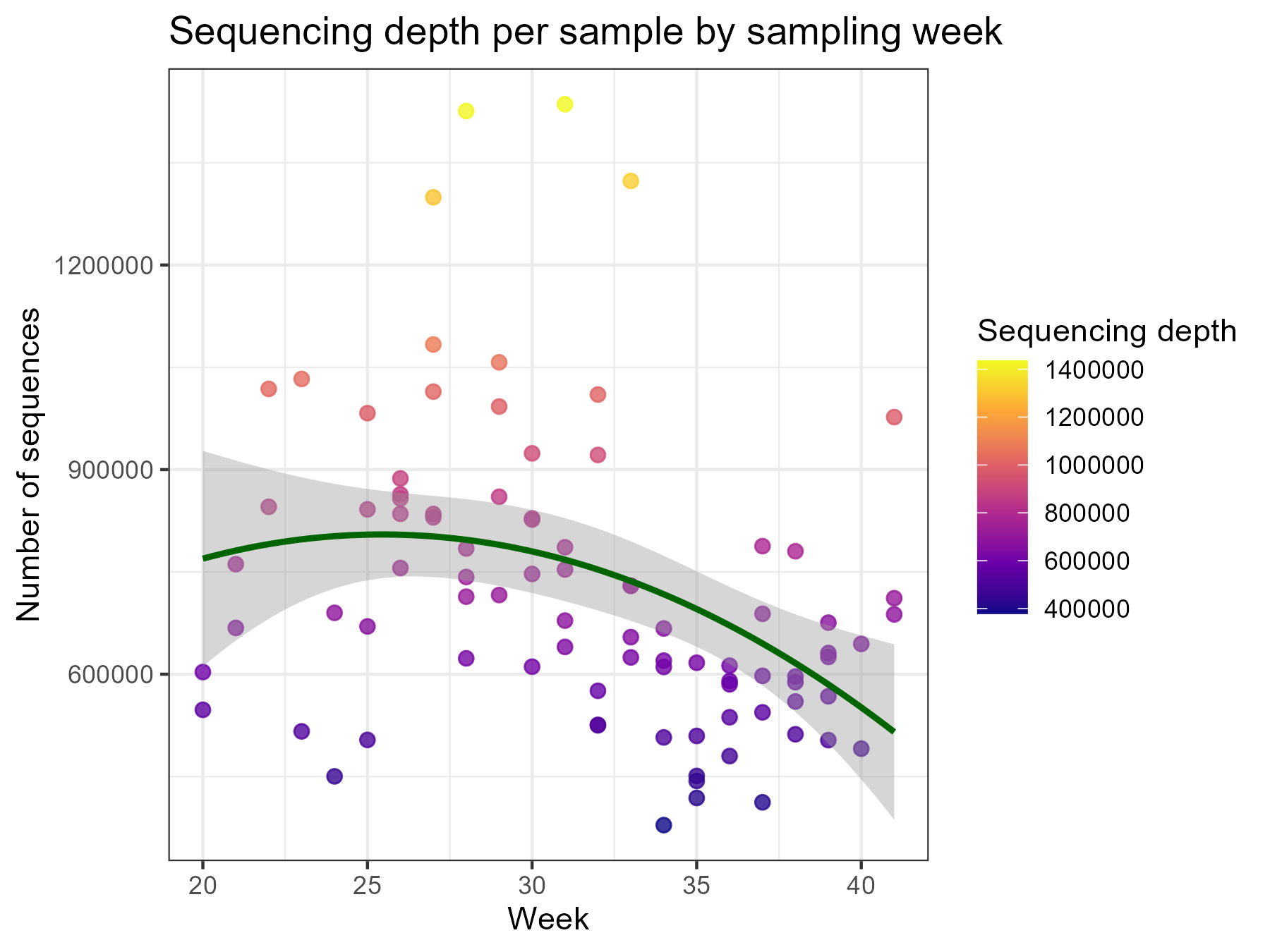
If we would like to test if the OTU richness differs between sampling seasons (spring, summer, autumn), then we would need to include sequencing depth as a covariate in the statistical analyses to separate the effect of sequencing depth from the effect of sampling season — even though all samples showed sufficient sequencing depth (rarefaction curves reached asymptote). If we would not include sequencing depth as a covariate, then the effect of sampling season would be confounded by the effect of sequencing depth (even when all samples reached asymptote, samples with higher depth can still have slightly higher observed OTU richness, so when depth differs between seasons the raw season effect on richness mixes biology with that technical effect).

---

Richness

Let’s further examine the number of OTUs across the altitudinal gradient.

Total OTU richness per altitude

#!/usr/bin/Rscript

library(tidyverse)

sample_names = colnames(OTU_table)

# OTU richness for a given altitude
richness_for_alt = function(alt) {
  these_samples = rownames(sample_metadata)[sample_metadata$altitude == alt]
  these_samples = intersect(these_samples, sample_names)

  if (length(these_samples) == 0) return(0L)

  mat = as.matrix(OTU_table[, these_samples, drop = FALSE])
  sum(rowSums(mat > 0) > 0)
}

# unique altitudes in sample metadata, sorted for plotting
alts = sort(unique(sample_metadata$altitude))

# create a dataframe with altitude and OTU richness
richness_by_altitude = tibble(
  altitude = alts,
  n_species = vapply(alts, richness_for_alt, integer(1))
)

# plot total richness vs altitude
p_tot = ggplot(richness_by_altitude,
                aes(x = altitude, y = n_species, group = 1)) +
  geom_line(aes(color = "Linear trend (lm)"), linewidth = 1) +
  geom_smooth(aes(color = "Linear trend (lm)"),
              method = "lm", se = TRUE,
              linewidth = 0.9, show.legend = FALSE) +
  geom_point(aes(color = "Altitude-specific richness"), size = 4) +
  geom_text(aes(label = n_species),
            vjust = -0.8, size = 3, color = "black") +
  scale_color_manual(
    name = "",
    values = c(
      "Altitude-specific richness" = "black",
      "Linear trend (lm)" = "lightblue"
    )
  ) +
  labs(
    title = "Total OTU richness across altitude",
    x = "Altitude (m)",
    y = "OTU richness"
  ) +
  theme_bw(base_size = 12) +
  theme(
    plot.title = element_text(face = "bold"),
    panel.grid.minor = element_blank(),
    legend.position = "bottom"
  )

# Save plot
ggsave(
  filename = file.path(results, "richness_by_altitude.png"),
  plot = p_tot,
  width = 5, height = 4.5, dpi = 300)

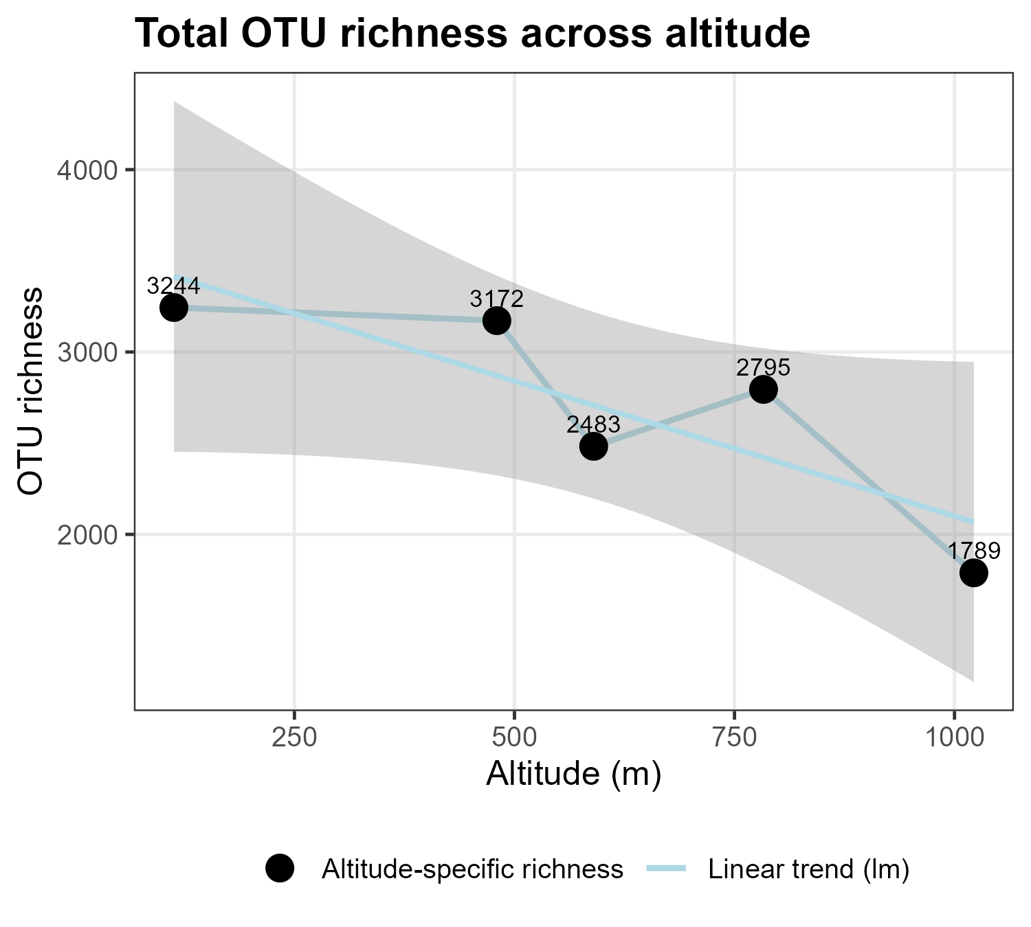
The resulting pattern suggests that total OTU richness tends to decline towards higher elevations. This is an expected pattern, as environmental stress increases with altitude, especially in the higher latitude regions (such as Norway in that example dataset).

Let’s test this relationship more formally.

Richness by altitude with linear and quadratic fits

#!/usr/bin/Rscript

# Use Generalized Linear Model (GLM) with negative binomial
# distribution to model the richness data.
# Negative binomial distribution is a common choice for count data
# with overdispersion (variance > mean).
library(MASS)

# log10 transform the sequencing_depth
sample_richness$log_sequencing_depth =
  log10(sample_richness$sequencing_depth)

# Fit linear and quadratic models (with altitude and sequencing depth)
glm_richness_linear = glm.nb(
  richness ~ altitude + log_sequencing_depth,
  data = sample_richness
)
glm_richness_quad = glm.nb(
  richness ~ poly(altitude, 2) + log_sequencing_depth,
  data = sample_richness
)

# Compare: is quadratic better than linear?
anova(glm_richness_linear, glm_richness_quad, test = "Chisq")
  # -> Pr(Chi = 0.0006887357


# Quadratic model summary (coefficients on log(mean richness) scale)
summary(glm_richness_quad)
#                        Estimate Std. Error z value Pr(>|z|)
#   (Intercept)            0.9717     1.9283   0.504 0.614320
#   poly(altitude, 2)1    -0.8119     0.3778  -2.149 0.031645 *
#   poly(altitude, 2)2    -1.3591     0.3765  -3.610 0.000307 ***
#   log_sequencing_depth   0.8727     0.3300   2.645 0.008175 **

## Deviance-based pseudo-R2
pseudo_R2_richness_quad =
  1 - (glm_richness_quad$deviance / glm_richness_quad$null.deviance)
cat("Pseudo-R2 (glm_richness_quad): ", round(pseudo_R2_richness_quad, 4), "\n")
  #-> Pseudo-R2 (glm_richness_quad):  0.2002

# Plot richness vs altitude with linear and quadratic fits
library(ggplot2)
p = ggplot(sample_richness,
                              aes(x = altitude, y = richness)) +
  geom_point(size = 3, alpha = 0.8) +
  geom_smooth(method = "lm", aes(linetype = "Linear"),
              color = "gray", se = F) +
  geom_smooth(method = "lm", formula = y ~ poly(x, 2),
              aes(linetype = "Quadratic"),
              color = "darkgreen", se = TRUE) +
  scale_linetype_manual(name = "Trend",
                        values = c(Linear = "dashed",
                                  Quadratic = "solid")) +
  labs(
    title = "OTU richness by altitude",
    x = "Altitude (m)",
    y = "OTU richness"
  ) +
  theme_bw()

ggsave(
  filename = file.path(results, "richness_by_altitude2.png"),
  plot = p,
  width = 6, height = 4.5, dpi = 300
)

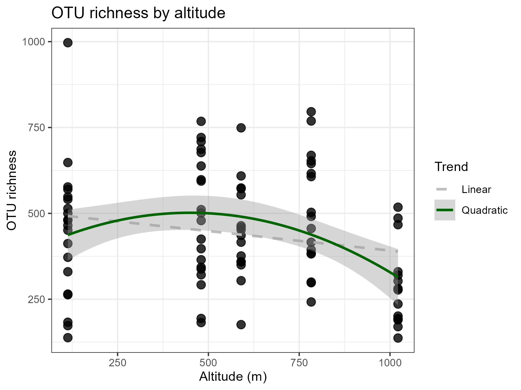
A negative-binomial GLM of OTU richness on altitude and sequencing depth was significantly improved by adding a quadratic altitude term (likelihood-ratio test p ≈ 0.0007). That is, OTU richness changes significantly across the altitudinal gradient, in a curved rather than linear way. The model explains about 20% of the null deviance in richness (pseudo-R2 = 0.20), so other potential drivers (e.g. habitat, season) are not captured in this model.

As we can notice from the plot above (and below), the per altitude richness is highly variable, and that originates from the sampling across 20 weeks at each altitude. Thus, let’s include seasonality into the model.

Model with altitude, sequencing depth, and seasonality

#!/usr/bin/Rscript

library(MASS)
# GLM for OTU richness with altitude, sequencing depth, and seasonality
glm_season = glm.nb(
  richness ~ poly(altitude, 2) +
    log_sequencing_depth +
    cos(2 * pi * week / 52) + # annual cycle as a cosine function
    sin(2 * pi * week / 52),  # annual cycle as a sin function
  data = sample_richness
)
summary(glm_season)
#->
#                          Estimate Std. Error  z value Pr(>|z|)
#   (Intercept)            2.11097    1.45721   1.449   0.147439
#   poly(altitude, 2)1    -1.04241    0.27319  -3.816   0.000136 ***
#   poly(altitude, 2)2    -1.30751    0.26214  -4.988   6.11e-07 ***
#   log_sequencing_depth   0.47899    0.25160   1.904   0.056946 .
#   cos(2 * pi * week/52) -1.18471    0.11981  -9.888   < 2e-16 ***
#   sin(2 * pi * week/52) -0.78676    0.09008  -8.734   < 2e-16 ***
#


## Compare glm_season to model without seasonal terms
# Deviance-based pseudo-R2:
pseudoR2_quad = 1 - (glm_richness_quad$deviance / glm_richness_quad$null.deviance)
pseudoR2_season = 1 - (glm_season$deviance / glm_season$null.deviance)

cat("Pseudo-R2 (quad):", pseudoR2_quad)
  #-> Pseudo-R2 (quad): 0.2001701
cat("Pseudo-R2 (season):", pseudoR2_season)
  #-> Pseudo-R2 (season): 0.6192453

## AIC comparison
AIC_quad = AIC(glm_richness_quad)
AIC_season = AIC(glm_season)
cat("AIC (quad):", AIC_quad)
  #-> AIC (quad): 1147.558
cat("AIC (season):", AIC_season)
  #-> AIC (season): 1085.174

## Compare using anova test (Likelihood Ratio Test)
anova(glm_richness_quad, glm_season, test = "Chisq")
  #-> Pr(Chi) = 3.885781e-15

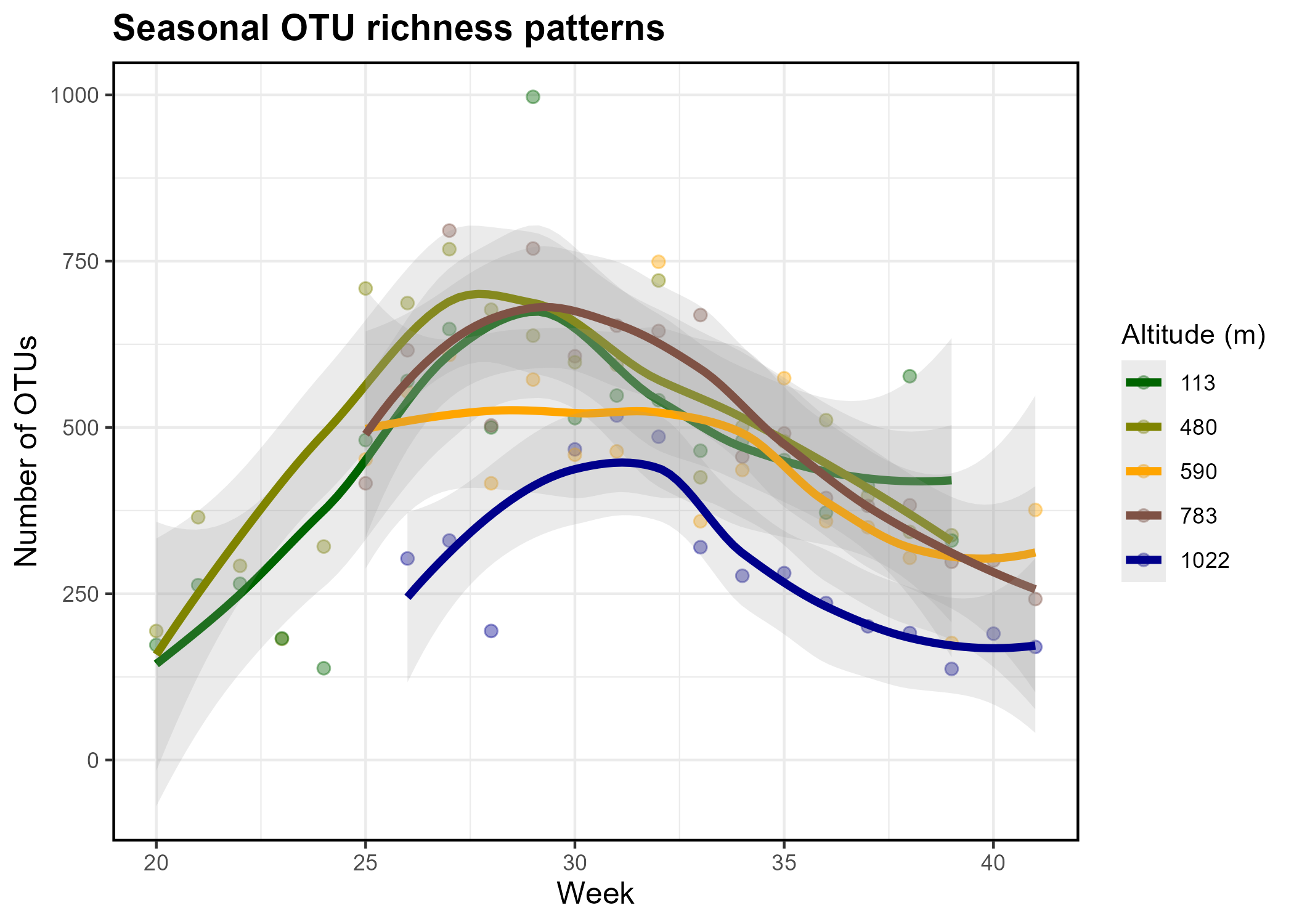
In addition to altitude, the seasonality (cosine and sine of week) is a significant driver of insect OTU richness (p < 0.0001). Comapred with model that did not have seasonality terms included, the model with seasonality had much higher pseudo-R2 (0.619 vs 0.200); indicating a substantial increase in the model’s explanatory power. This increase was not simply due to overfitting, as the likelihood-ratio test shows that the model with seasonality fits significantly better than the model without it (p < 0.0001), had lower AIC (1085 vs 1148).

---