Hierarchical Modelling of Species Communities
Hierarchical Modelling of Species Communities (HMSC) is a framework for Joint Species Distribution Modelling; a model-based approach for analyzing community ecological data (Ovaskainen et al.2017).
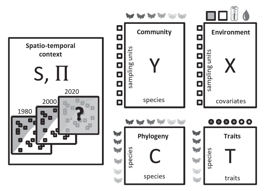
The input data for HMSC-analyses includes a matrix of species occurrences or abundances and a matrix of environmental covariates (sampling units as rows). Optionally additional input data include species traits and phylogeny, and information about the spatiotemporal context of the sampling design. HMSC yields inference both at species and community levels.
Starting point
The input for HMSC analysis consists of species/OTU community matrix (Y matrix) accompanied with the matrix of environmental covariates (X matrix), and optionally species traits (T) matrix and phylogeny (C) matrix.
Traits
Including the traits matrix helps to understand how species-specific traits influence the community assebly processes. Traits matrix may include data for example about body size, shape, feeding type, etc.
body_size |
shape |
trophic_guild |
|
OTU_01 |
2 |
square |
1 |
OTU_02 |
2 |
round |
1 |
OTU_03 |
0.1 |
round |
2 |
OTU_04 |
0.2 |
variable |
3 |
Phylogeny
Including the phylogeny matrix helps to understand if the species responses to the environmental covariates are phylogenetically structured, i.e., do similar species respond similarly.
The phylogeny matrix may be presented as Newick tree file. Alternatively, data on taxonomic ranks may used as a proxy of phylogenetic relatedness. In the latter case, the UNCLASSIFIED taxonomic ranks (that are common in the metabarcoding data) should be informative in a sense that not all e.g. family level unclassified OTUs would be considered as closely related because they have the ‘same label’. For example, the distance between unclassified OTUs could be calculated and then OTUs falling within the user defined distance threshold could be classified as various levels of pseudotaxa.
Example of the taxonomy table:
… |
Class |
Order |
Family |
Genus |
|
OTU_01 |
… |
Collembola |
Entomobryomorpha |
Entomobryidae |
Entomobrya |
OTU_02 |
… |
Collembola |
Entomobryomorpha |
Family_0032 |
Genus_001 |
OTU_03 |
… |
Collembola |
Entomobryomorpha |
Isotomidae |
Parisotoma |
OTU_04 |
… |
Collembola |
Entomobryomorpha |
Family_0032 |
Genus_022 |
Here, for example the sequences of OTU_02 and OTU_04 differ 9.8%; so we consider those are originating from different genera but likely from the same family.
Install HMSC
Install hmsc R package (if already not installed).
 1#!/usr/bin/Rscript
 2
 3# install 'devtools'; if not yet installed
 4install.packages("devtools")
 5library(devtools)
 6
 7# install hmsc package
 8install_github("hmsc-r/HMSC")
 9
10# load hmsc
11library(Hmsc)
12
13# check the version
14packageVersion("Hmsc")
Select data
In this ‘select data’ section, we are assuming that our input Y and X matrixes are tab delimited text files where samples are in rows; and taxonomy table format follows the above example.
Here, we are also deciding if we want to proceed with the presence-absence or abundance (read count) community matrix.
Note
Before using to the full dataset, try fitting the model with a small subset for faster model testing and validation.
 1#!/usr/bin/Rscript
 2
 3# input matrices file names; according to the above HMSC figure.
 4   # here, expecting all files to be tab-delimited.
 5Y_file = "OTU_table.txt" # Community; samples are rows
 6X_file = "env_meta.txt"  # Environment; samples are rows
 7C_file = "taxonomy.txt"  # Phylogeny (optional)
 8                         # (herein a 'pseudo-phylogeny' based on the
 9                         # assigned taxonomic ranks; species are rows)
10T_file = ""              # Traits (optional)
11sp_prevalence = 100      # set a species prevalence threshold;
12                         # meaning that perform HMSC for species
13                         # in a Y-matrix, that occur >= 100 samples in this case.
14 #-------------------------------------------------------------------------------------------#
15
16 # load community matrix Y
17 Y = read.table(Y_file, sep = "\t",
18                   check.names = F,
19                   header = T,
20                   row.names = 1)
21 # load metadata matrix X
22 X = read.table(X_file, sep = "\t",
23                     check.names = F,
24                     header = T,
25                     row.names = 1)
26 # load taxonomy matrix C;
27   # so we can use it as a proxy for phylogeny
28 taxonomy = read.table(C_file, sep = "\t",
29                       check.names = F,
30                       header = T,
31                       row.names = 1)
32
33 # herein, converting Y matrix to presence-absence
34 Y = 1*(Y>0)
35
36 # select OTUs/species that are present at least in $sp_prevalence (specified above) samples
37 prevalence = colSums(Y != 0)
38 select.sp = prevalence >= sp_prevalence
39 Y = Y[, select.sp]
40 taxonomy = taxonomy[select.sp, ]
41
42 ### creating a phylogenetic tree from a set of nested taxonomic ranks in the taxonomy table
43  # ranks as.factors; assuming that ranks start from the 2nd column in the taxonomy table
44     # and we have 7 ranks
45 for(i in 2:8) taxonomy[,i] = as.factor(taxonomy[,i])
46  # convert tax to phylo tree
47 phy.tree = as.phylo(~Phylum/Class/Order/Family/Genus/Species,
48                 data = taxonomy, collapse = FALSE)
49
50 # this "pseudo-tree" does not have any branch lengths, which are needed for the model;
51 # assign arbitrary branch lengths
52   if (is.null(phy.tree$edge.length)) {
53     phy.tree$edge.length = rep(1, nrow(phy.tree$edge))
54   }
55  # rename tree tip lables according to the labels in the Y matrix.
56  phy.tree$tip.label = colnames(Y)
57
58  # check the tree
59  plot(phy.tree, cex=0.6)
Define model
According to our dataset, we are defining the model for HMSC. That is, we specify the structure, including the response variable (community data), covariates (environmental predictors), random effects, and phylogenetic relationships.
 1#!/usr/bin/Rscript
 2
 3library(Hmsc)
 4
 5 # defining our study design; structure of the data
 6 studyDesign = data.frame(
 7                 sample = as.factor(rownames(X)),    # rownames(X) = sample names
 8                 site = as.factor(X$Site)
 9                 )
10
11 ### incorporating random effects into the  HMSC model.
12  # (to capture the influence of unmeasured factors that vary across different
13  # levels of the data; e.g., among sites, samples).
14 # sampling units
15 rL.sample = HmscRandomLevel(units = levels(studyDesign$sample))
16 # sampling sites
17 rL.site = HmscRandomLevel(units = levels(studyDesign$site))
18
19 # convert sample collection dates into Julian days relative to a specific start date
20 da = as.Date(meta$CollectionDate)
21 jday = 1 + julian(da) - julian(as.Date("2024-01-01"))
22
23 # not covered here, but DOWNLOAD RELEVANT COVARIATES (E.G., CLIMATE, WEATHER, LANDCOVER)
24 # FROM DATABASES BASED ON COORDINATES AND SAMPLING TIMES
25
26 # create a data frame of covariates (predictor variables) that will be included in the model
27 XData = data.frame(seqdepth = log(meta$seq_depth),  # number of sequences per sample
28                     jday)                           # Julian days
29
30 ### specify the formula for the fixed effects
31 # using 3.141593 instead of pi to prevent issues when 'pi' is considered as a variable;
32 XFormula = ~cos(2*3.141593*jday/365) +  # model seasonal effects; annual cycles
33             sin(2*3.141593*jday/365) +  # model seasonal effects; annual cycles
34             cos(4*3.141593*jday/365) +  # model seasonal effects; semiannual cycles
35             sin(4*3.141593*jday/365) +  # model seasonal effects; semiannual cycles
36             seqdepth                    # number of sequences per sample
37
38 ### define a model
39 m = Hmsc(Y = Y,             # response matrix
40       distr = "probit",      # distribution model for the response variable ('probit' for PA)
41       XData = XData,          # predictor variables
42       XFormula = XFormula,     # fixed effects in the model
43       phyloTree = phy.tree,     # phylogenetic tree object
44       studyDesign = studyDesign, # study design object
45       ranLevels = list(sample = rL.sample, site = rL.site)) # random level objects
46
47 # organize, name, and save your HMSC models (to easily manage multiple models if needed)
48 models = list(m)
49 names(models) = c("model_1")
50 save(models, file = paste0("models/unfitted_models.RData"))
51
52 # check models
53 models
Fit model
The following HMSC pipeline is a modified version of the pipeline presented at the ISEC 2024 Hmsc workshop.
input:
Unfitted_models file (unfitted_models.RData)
output:
 1#!/usr/bin/Rscript
 2
 3# set working directory
 4localDir = "."
 5# specify 'models' dir (input/output dir)
 6modelDir = file.path(localDir, "models")
 7
 8# load input (unfitted_models)
 9load(file=file.path(modelDir,"unfitted_models.RData"))
10
11# number of parallel chains (CPUs) for MCMC sampling
12nParallel = NULL   # if NULL, then nParallel = nChains
13
14# number of samples and thinning intervals for each iteration
15samples_list = c(5, 250, 250, 250, 250, 250)   # number of iterations of the MCMC
16thin_list = c(1, 1, 10, 100, 1000, 10000)      # thinning interval;  keep every k-th sample
17# number of MCMC chains
18nChains = 4
19#-------------------------------------------------------------------------------------------#
20
21library(Hmsc)
22
23# iterate over sample and thin lists to fit models with different configurations
24nm = length(models)  # number of models (for loop)
25if(is.null(nParallel)) nParallel = nChains
26Lst = 1
27while(Lst <= length(samples_list)){
28  thin = thin_list[Lst]
29  samples = samples_list[Lst]
30  print(paste0("thin = ",as.character(thin),"; samples = ", as.character(samples)))
31  filename = file.path(modelDir,paste("models_thin_", as.character(thin),
32                                            "_samples_", as.character(samples),
33                                            "_chains_", as.character(nChains),
34                                            ".Rdata", sep = ""))
35  if(file.exists(filename)){
36    print("model had been fitted already")
37  } else {
38    print(date())
39    for (mi in 1:nm) {
40      print(paste0("model = ",names(models)[mi]))
41      m = models[[mi]]
42      m = sampleMcmc(m, samples = samples, thin=thin,
43                    adaptNf=rep(ceiling(0.4*samples*thin), m$nr),
44                    transient = ceiling(0.5*samples*thin),
45                    nChains = nChains,
46                    nParallel = nParallel)
47      models[[mi]] = m
48    }
49    save(models, file=filename)
50  }
51  Lst = Lst + 1
52}
Evaluate convergence
Evaluating convergence ensures the accuracy and reliability of the model’s results by confirming that the MCMC algorithm has adequately explored the parameter space and that the chains have stabilized.
input:
Fitted models directory models.
Check the input path, and typically other parts of the scripts do not need modifications.
output:
MCMC convergence statistics for selected model parameters, illustrated (for all runs) in the file “results/MCMC_convergence.pdf”, and the text file “results/MCMC_convergence.txt”.
  1#!/usr/bin/Rscript
  2
  3library(Hmsc)
  4library(colorspace)
  5library(vioplot)
  6
  7# make the script reproducible
  8set.seed(1)
  9
 10# set working directory
 11localDir = "."
 12# specify 'models' dir (input dir)
 13modelDir = file.path(localDir, "models")
 14# specify 'results' dir (output dir)
 15resultDir = file.path(localDir, "results")
 16if (!dir.exists(resultDir)) dir.create(resultDir)
 17
 18# number of samples and thinning intervals for each iteration (AS ABOVE)
 19samples_list = c(5, 250, 250, 250, 250, 250)   # number of iterations of the MCMC
 20thin_list = c(1, 1, 10, 100, 1000, 10000)      # thinning interval;  keep every k-th sample
 21# number of MCMC chains
 22nChains = 4
 23#-------------------------------------------------------------------------------------------#
 24
 25# setting commonly adjusted parameters
 26showBeta = TRUE  # default = TRUE, converg. shown for beta-parameters
 27showGamma = TRUE # default = FALSE, converg. not shown for gamma-parameters
 28showOmega = TRUE # default = FALSE, converg. not shown for Omega-parameters
 29maxOmega = 100   # default = 50, converg. of Omega shown for 50 randomly selected species pairs
 30showRho = TRUE   # default = FALSE, converg. not shown for rho-parameters
 31showAlpha = TRUE # default = FALSE, converg. not shown for alpha-parameters
 32
 33# set up a text file to store MCMC convergence statistics
 34text.file = file.path(resultDir,"/MCMC_convergence.txt")
 35cat("MCMC Convergennce statistics\n\n", file = text.file, sep="")
 36
 37ma.beta = NULL
 38na.beta = NULL
 39ma.gamma = NULL
 40na.gamma = NULL
 41ma.omega= NULL
 42na.omega = NULL
 43ma.alpha = NULL
 44na.alpha = NULL
 45ma.rho = NULL
 46na.rho = NULL
 47Lst = 1
 48while(Lst <= nst){
 49  thin = thin_list[Lst]
 50  samples = samples_list[Lst]
 51
 52  filename = file.path(modelDir,paste("models_thin_", as.character(thin),
 53                                      "_samples_", as.character(samples),
 54                                      "_chains_",as.character(nChains),
 55                                      ".Rdata",sep = ""))
 56  if(file.exists(filename)){
 57    load(filename)
 58    cat(c("\n",filename,"\n\n"),file=text.file,sep="",append=TRUE)
 59    nm = length(models)
 60    for(j in 1:nm){
 61      mpost = convertToCodaObject(models[[j]], spNamesNumbers = c(T,F), covNamesNumbers = c(T,F))
 62      nr = models[[j]]$nr
 63      cat(c("\n",names(models)[j],"\n\n"),file=text.file,sep="",append=TRUE)
 64      if(showBeta){
 65        psrf = gelman.diag(mpost$Beta,multivariate=FALSE)$psrf
 66        tmp = summary(psrf)
 67        cat("\nbeta\n\n",file=text.file,sep="",append=TRUE)
 68        cat(tmp[,1],file=text.file,sep="\n",append=TRUE)
 69        if(is.null(ma.beta)){
 70          ma.beta = psrf[,1]
 71          na.beta = paste0(as.character(thin),",",as.character(samples))
 72        } else {
 73          ma.beta = cbind(ma.beta,psrf[,1])
 74          if(j==1){
 75            na.beta = c(na.beta,paste0(as.character(thin),",",as.character(samples)))
 76          } else {
 77            na.beta = c(na.beta,"")
 78          }
 79        }
 80      }
 81      if(showGamma){
 82        psrf = gelman.diag(mpost$Gamma,multivariate=FALSE)$psrf
 83        tmp = summary(psrf)
 84        cat("\ngamma\n\n",file=text.file,sep="",append=TRUE)
 85        cat(tmp[,1],file=text.file,sep="\n",append=TRUE)
 86        if(is.null(ma.gamma)){
 87          ma.gamma = psrf[,1]
 88          na.gamma = paste0(as.character(thin),",",as.character(samples))
 89        } else {
 90          ma.gamma = cbind(ma.gamma,psrf[,1])
 91          if(j==1){
 92            na.gamma = c(na.gamma,paste0(as.character(thin),",",as.character(samples)))
 93          } else {
 94            na.gamma = c(na.gamma,"")
 95          }
 96        }
 97      }
 98      if(showRho & !is.null(mpost$Rho)){
 99        psrf = gelman.diag(mpost$Rho,multivariate=FALSE)$psrf
100        cat("\nrho\n\n",file=text.file,sep="",append=TRUE)
101        cat(psrf[1],file=text.file,sep="\n",append=TRUE)
102      }
103      if(showOmega & nr>0){
104        cat("\nomega\n\n",file=text.file,sep="",append=TRUE)
105        for(k in 1:nr){
106          cat(c("\n",names(models[[j]]$ranLevels)[k],"\n\n"),file=text.file,sep="",append=TRUE)
107          tmp = mpost$Omega[[k]]
108          z = dim(tmp[[1]])[2]
109          if(z > maxOmega){
110            sel = sample(1:z, size = maxOmega)
111            for(i in 1:length(tmp)){
112              tmp[[i]] = tmp[[i]][,sel]
113            }
114          }
115          psrf = gelman.diag(tmp, multivariate = FALSE)$psrf
116          tmp = summary(psrf)
117          cat(tmp[,1],file=text.file,sep="\n",append=TRUE)
118          if(is.null(ma.omega)){
119            ma.omega = psrf[,1]
120            na.omega = paste0(as.character(thin),",",as.character(samples))
121          } else {
122            ma.omega = cbind(ma.omega,psrf[,1])
123            if(j==1){
124              na.omega = c(na.omega,paste0(as.character(thin),",",as.character(samples)))
125            } else {
126              na.omega = c(na.omega,"")
127            }
128          }
129        }
130      }
131      if(showAlpha & nr>0){
132        for(k in 1:nr){
133          if(models[[j]]$ranLevels[[k]]$sDim>0){
134            cat("\nalpha\n\n",file=text.file,sep="\n",append=TRUE)
135            cat(c("\n",names(models[[j]]$ranLevels)[k],"\n\n"),file=text.file,sep="",append=TRUE)
136            psrf = gelman.diag(mpost$Alpha[[k]],multivariate = FALSE)$psrf
137            cat(psrf[,1],file=text.file,sep="\n",append=TRUE)
138          }
139        }
140      }
141    }
142  }
143  Lst = Lst + 1
144}
145
146pdf(file= file.path(resultDir,"/MCMC_convergence.pdf"))
147if(showBeta){
148  par(mfrow=c(2,1))
149  vioplot(ma.beta,col=rainbow_hcl(nm),names=na.beta,ylim=c(0,max(ma.beta)),main="psrf(beta)")
150  legend("topright",legend = names(models), fill=rainbow_hcl(nm))
151  vioplot(ma.beta,col=rainbow_hcl(nm),names=na.beta,ylim=c(0.9,1.1),main="psrf(beta)")
152}
153if(showGamma){
154  par(mfrow=c(2,1))
155  vioplot(ma.gamma,col=rainbow_hcl(nm),names=na.gamma,ylim=c(0,max(ma.gamma)),main="psrf(gamma)")
156  legend("topright",legend = names(models), fill=rainbow_hcl(nm))
157  vioplot(ma.gamma,col=rainbow_hcl(nm),names=na.gamma,ylim=c(0.9,1.1),main="psrf(gamma)")
158}
159if(showOmega & !is.null(ma.omega)){
160  par(mfrow=c(2,1))
161  vioplot(ma.omega,col=rainbow_hcl(nm),names=na.omega,ylim=c(0,max(ma.omega)),main="psrf(omega)")
162  legend("topright",legend = names(models), fill=rainbow_hcl(nm))
163  vioplot(ma.omega,col=rainbow_hcl(nm),names=na.omega,ylim=c(0.9,1.1),main="psrf(omega)")
164}
165dev.off()
check the diagnostics
We need to confirm that the MCMC chain has converged. If the chains have not converged, the samples privided by the MCMC chain can yield biased parameter estimates.
Compute model fit
Assessing the model’s performance and validating its accuracy. …
input:
Fitted models directory models.
Check the input path, and typically other parts of the scripts do not need modifications.
output:
 1#!/usr/bin/Rscript
 2
 3library(Hmsc)
 4
 5# make the script reproducible
 6set.seed(1)
 7
 8# set working directory
 9localDir = "."
10# specify 'models' dir (input/output dir)
11modelDir = file.path(localDir, "models")
12
13# number of samples and thinning intervals for each iteration (AS ABOVE)
14samples_list = c(5, 250, 250, 250, 250, 250)   # number of iterations of the MCMC
15thin_list = c(1, 1, 10, 100, 1000, 10000)      # thinning interval;  keep every k-th sample
16# number of MCMC chains
17nChains = 4
18
19# number of parallel chains (CPUs) for MCMC sampling
20nParallel = NULL   # if NULL, then nParallel = nChains
21# number of cross-validations
22nfolds = 2         # default: (2) two-fold cross-validation
23#-------------------------------------------------------------------------------------------#
24
25if(is.null(nParallel)) nParallel = nChains
26Lst = 1
27while(Lst <= length(samples_list)){
28  thin = thin_list[Lst]
29  samples = samples_list[Lst]
30  filename.in = file.path(modelDir,paste("models_thin_", as.character(thin),
31                                        "_samples_", as.character(samples),
32                                        "_chains_",as.character(nChains),
33                                        ".Rdata",sep = ""))
34  filename.out = file.path(modelDir,paste("MF_thin_", as.character(thin),
35                                          "_samples_", as.character(samples),
36                                          "_chains_",as.character(nChains),
37                                          "_nfolds_", as.character(nfolds),
38                                          ".Rdata",sep = ""))
39  if(file.exists(filename.out)){
40    print(paste0("thin = ",as.character(thin),"; samples = ",as.character(samples)))
41    print("model fit had been computed already")
42  } else {
43    if(file.exists(filename.in)){
44      print(paste0("thin = ",as.character(thin),"; samples = ",as.character(samples)))
45      print(date())
46      load(file = filename.in) #models
47      nm = length(models)
48
49      MF = list()
50      MFCV = list()
51      WAIC = list()
52
53      for(mi in 1:nm){
54        print(paste0("model = ",names(models)[mi]))
55        m = models[[mi]]
56        preds = computePredictedValues(m)
57        MF[[mi]] = evaluateModelFit(hM=m, predY=preds)
58        partition = createPartition(m, nfolds = nfolds) #USE column = ...
59        preds = computePredictedValues(m,partition=partition, nParallel = nParallel)
60        MFCV[[mi]] = evaluateModelFit(hM=m, predY=preds)
61        WAIC[[mi]] = computeWAIC(m)
62      }
63      names(MF)=names(models)
64      names(MFCV)=names(models)
65      names(WAIC)=names(models)
66
67      save(MF,MFCV,WAIC,file = filename.out)
68    }
69  }
70  Lst = Lst + 1
71}
Show model fit
Evaluate and visualize the model fit for different thinning and sampling configurations.
input:
Fitted models directory models.
Check the input path, and typically other parts of the scripts do not need modifications.
output:
Model fits illustrated (for highest RUN of compute model fit) in the file results/model_fit.pdf.
  1#!/usr/bin/Rscript
  2
  3library(Hmsc)
  4
  5# make the script reproducible
  6set.seed(1)
  7
  8# set working directory
  9localDir = "."
 10# specify 'models' dir (input dir)
 11modelDir = file.path(localDir, "models")
 12# specify 'results' dir (output dir)
 13resultDir = file.path(localDir, "results")
 14if (!dir.exists(resultDir)) dir.create(resultDir)
 15
 16# number of samples and thinning intervals for each iteration (AS ABOVE)
 17samples_list = c(5, 250, 250, 250, 250, 250)   # number of iterations of the MCMC
 18thin_list = c(1, 1, 10, 100, 1000, 10000)      # thinning interval;  keep every k-th sample
 19# number of MCMC chains
 20nChains = 4
 21
 22# number of cross-validations
 23nfolds = 2         # default: (2) two-fold cross-validation
 24#-------------------------------------------------------------------------------------------#
 25
 26for (Lst in nst:1) {
 27  thin = thin_list[Lst]
 28  samples = samples_list[Lst]
 29
 30  filename = file.path(modelDir,paste("MF_thin_", as.character(thin),
 31                                      "_samples_", as.character(samples),
 32                                      "_chains_",as.character(nChains),
 33                                      "_nfolds_", as.character(nfolds),
 34                                      ".Rdata",sep = ""))
 35  if(file.exists(filename)){break}
 36}
 37if(file.exists(filename)){
 38  load(filename)
 39
 40  nm = length(MF)
 41  modelnames = names(MF)
 42  pdf(file = file.path(resultDir,paste0("/model_fit_nfolds_",nfolds,".pdf")))
 43  for(j in 1:nm){
 44    cMF = MF[[j]]
 45    cMFCV = MFCV[[j]]
 46    if(!is.null(cMF$TjurR2)){
 47      plot(cMF$TjurR2,cMFCV$TjurR2,xlim=c(-1,1),ylim=c(-1,1),
 48          xlab = "explanatory power",
 49          ylab = "predictive power",
 50          main=paste0(modelnames[j],", thin = ",
 51                      as.character(thin),
 52                      ", samples = ",as.character(samples),
 53                      ": Tjur R2.\n",
 54                      "mean(MF) = ",as.character(mean(cMF$TjurR2,na.rm=TRUE)),
 55                      ", mean(MFCV) = ",as.character(mean(cMFCV$TjurR2,na.rm=TRUE))))
 56      abline(0,1)
 57      abline(v=0)
 58      abline(h=0)
 59    }
 60    if(!is.null(cMF$R2)){
 61      plot(cMF$R2,cMFCV$R2,xlim=c(-1,1),ylim=c(-1,1),
 62          xlab = "explanatory power",
 63          ylab = "predictive power",
 64          main=paste0(modelnames[[j]],", thin = ",as.character(thin),
 65                      ", samples = ",as.character(samples),
 66                      ": R2. \n",
 67                      "mean(MF) = ",as.character(mean(cMF$R2,na.rm=TRUE)),
 68                      ", mean(MFCV) = ",as.character(mean(cMFCV$R2,na.rm=TRUE))))
 69      abline(0,1)
 70      abline(v=0)
 71      abline(h=0)
 72    }
 73    if(!is.null(cMF$AUC)){
 74      plot(cMF$AUC,cMFCV$AUC,xlim=c(0,1),ylim=c(0,1),
 75          xlab = "explanatory power",
 76          ylab = "predictive power",
 77          main=paste0(modelnames[[j]],", thin = ",as.character(thin),
 78                      ", samples = ",as.character(samples),
 79                      ": AUC. \n",
 80                      "mean(MF) = ",as.character(mean(cMF$AUC,na.rm=TRUE)),
 81                      ", mean(MFCV) = ",as.character(mean(cMFCV$AUC,na.rm=TRUE))))
 82      abline(0,1)
 83      abline(v=0.5)
 84      abline(h=0.5)
 85    }
 86    if(FALSE && !is.null(cMF$O.TjurR2)){
 87      plot(cMF$O.TjurR2,cMFCV$O.TjurR2,xlim=c(-1,1),ylim=c(-1,1),
 88          xlab = "explanatory power",
 89          ylab = "predictive power",
 90          main=paste0(modelnames[[j]],", thin = ",as.character(thin),", samples = ",as.character(samples),": O.Tjur R2"))
 91      abline(0,1)
 92      abline(v=0)
 93      abline(h=0)
 94    }
 95    if(FALSE && !is.null(cMF$O.AUC)){
 96      plot(cMF$O.AUC,cMFCV$O.AUC,xlim=c(0,1),ylim=c(0,1),
 97          xlab = "explanatory power",
 98          ylab = "predictive power",
 99          main=paste0(modelnames[[j]],", thin = ",as.character(thin),", samples = ",as.character(samples),": O.AUC"))
100      abline(0,1)
101      abline(v=0.5)
102      abline(h=0.5)
103    }
104    if(!is.null(cMF$SR2)){
105      plot(cMF$SR2,cMFCV$SR2,xlim=c(-1,1),ylim=c(-1,1),
106          xlab = "explanatory power",
107          ylab = "predictive power",
108          main=paste0(modelnames[[j]],", thin = ",as.character(thin),
109                      ", samples = ",as.character(samples),
110                      ": SR2. \n",
111                      "mean(MF) = ",as.character(mean(cMF$SR2,na.rm=TRUE)),
112                      ", mean(MFCV) = ",as.character(mean(cMFCV$SR2,na.rm=TRUE))))
113      abline(0,1)
114      abline(v=0)
115      abline(h=0)
116    }
117    if(FALSE && !is.null(cMF$C.SR2)){
118      plot(cMF$C.SR2,cMFCV$C.SR2,xlim=c(-1,1),ylim=c(-1,1),
119          xlab = "explanatory power",
120          ylab = "predictive power",
121          main=paste0(modelnames[[j]],", thin = ",as.character(thin),", samples = ",as.character(samples),": C.SR2"))
122      abline(0,1)
123      abline(v=0)
124      abline(h=0)
125    }
126  }
127  dev.off()
128}
Show parameter estimates
Assessing the model’s performance and validating its accuracy. …
input:
Fitted models directory models.
Check the input path, and typically other parts of the scripts do not need modifications.
output:
  1#!/usr/bin/Rscript
  2
  3library(Hmsc)
  4library(colorspace)
  5library(corrplot)
  6library(writexl)
  7
  8# make the script reproducible
  9set.seed(1)
 10
 11# set working directory
 12localDir = "."
 13# specify 'models' dir (input dir)
 14modelDir = file.path(localDir, "models")
 15# specify 'results' dir (output dir)
 16resultDir = file.path(localDir, "results")
 17if (!dir.exists(resultDir)) dir.create(resultDir)
 18
 19# number of samples and thinning intervals for each iteration (AS ABOVE)
 20samples_list = c(5, 250, 250, 250, 250, 250)   # number of iterations of the MCMC
 21thin_list = c(1, 1, 10, 100, 1000, 10000)      # thinning interval;  keep every k-th sample
 22# number of MCMC chains
 23nChains = 4
 24
 25# thresholds for the posterior support levels
 26support.level.beta = 0.95       # default: 0.95
 27support.level.gamma = 0.95      # default: 0.95
 28support.level.omega = 0.9       # default: 0.9
 29
 30
 31var.part.order.explained = NULL # default: in variance partitioning of explained variance,
 32                                #     species are shown in the order they are in the model.
 33  # -> use var.part.order.explained to select which order species are shown in the
 34  #                                                       raw variance partitioning.
 35  # var.part.order.raw should be a list of length the number of models.
 36  # for each element provide either 0 (use default);
 37  # or a vector of species indices;
 38  # or "decreasing" if you wish to order according to explanatory power
 39  # var.part.order.explained = list()
 40  # var.part.order.explained[[1]] = 0
 41  # var.part.order.explained[[2]] = c(2,1)
 42
 43var.part.order.raw = NULL       # default: in variance partitioning of raw variance, species
 44                                #              are shown in the order they are in the model.
 45  # -> use var.part.order.raw to select which order species are shown in the
 46  #                                           explained variance partitioning.
 47  # same options apply as for var.part.order.explained
 48  # var.part.order.raw = list()
 49  # var.part.order.raw[[1]] = "decreasing"
 50  # var.part.order.raw[[2]] = c(1,2)
 51
 52
 53show.sp.names.beta = NULL    # default: species names shown in beta plot if there are at
 54                             #                          most 30 species and no phylogeny
 55  # -> use show.sp.names.beta to choose to show / not show species names in betaPlot
 56  # if given, show.sp.names.beta should be a vector with length equalling number of models
 57  # show.sp.names.beta = c(TRUE,FALSE)
 58
 59plotTree = NULL              # default: tree is plotted in Beta plot if the model includes it.
 60  # -> use plotTree to choose to plot / not plot the tree in betaPlot.
 61  # if given, plotTree should be a vector with length equalling number of models
 62  # plotTree = c(FALSE,FALSE)
 63
 64omega.order = NULL           # default: species shown in the order they are in the model.
 65  # -> use omega.order to select which order species are shown in omega plots
 66  # omega.order should be a list of length the number of models.
 67  # for each element provide either 0 (use default);
 68  # or a vector of species indices;
 69  # or "AOE" if you wish to use the angular order of the eigenvectors.
 70  # omega.order = list()
 71  # omega.order[[1]] = "AOE"
 72  # omega.order[[2]] = c(2,1)
 73
 74show.sp.names.omega = NULL   # default: species names shown in beta plot if there are at
 75                             #                                           most 30 species.
 76  # show.sp.names.omega = c(TRUE,FALSE)
 77#-------------------------------------------------------------------------------------------#
 78
 79
 80text.file = file.path(resultDir,"/parameter_estimates.txt")
 81cat(c("This file contains additional information regarding parameter estimates.","\n","\n",
 82                                                                   sep=""), file=text.file)
 83
 84for (Lst in nst:1) {
 85  thin = thin_list[Lst]
 86  samples = samples_list[Lst]
 87  filename = file.path(modelDir,paste("models_thin_", as.character(thin),
 88                                      "_samples_", as.character(samples),
 89                                      "_chains_",as.character(nChains),
 90                                      ".Rdata",sep = ""))
 91  if(file.exists(filename)){break}
 92}
 93if(file.exists(filename)){
 94  load(filename)
 95  cat(c("\n",filename,"\n","\n"),file=text.file,sep="",append=TRUE)
 96  nm = length(models)
 97  if(is.null(var.part.order.explained)){
 98    var.part.order.explained = list()
 99    for(j in 1:nm) var.part.order.explained[[j]] = 0
100  }
101  if(is.null(var.part.order.raw)){
102    var.part.order.raw = list()
103    for(j in 1:nm) var.part.order.raw[[j]] = 0
104  }
105  if(is.null(omega.order)){
106    omega.order = list()
107    for(j in 1:nm) omega.order[[j]] = 0
108  }
109
110  modelnames = names(models)
111
112  pdf(file= file.path(resultDir,"parameter_estimates.pdf"))
113  for(j in 1:nm){
114    cat(c("\n",names(models)[j],"\n","\n"),file=text.file,sep="",append=TRUE)
115    m = models[[j]]
116    if(m$XFormula=="~."){
117      covariates = colnames(m$X)[-1]
118    } else {
119      covariates = attr(terms(m$XFormula),"term.labels")
120    }
121    if(m$nr+length(covariates)>1 & m$ns>1){
122      preds = computePredictedValues(m)
123      VP = computeVariancePartitioning(m)
124      vals = VP$vals
125      mycols = rainbow(nrow(VP$vals))
126      MF = evaluateModelFit(hM=m, predY=preds)
127      R2 = NULL
128      if(!is.null(MF$TjurR2)){
129        TjurR2 = MF$TjurR2
130        vals = rbind(vals,TjurR2)
131        R2=TjurR2
132      }
133      if(!is.null(MF$R2)){
134        R2=MF$R2
135        vals = rbind(vals,R2)
136      }
137      if(!is.null(MF$SR2)){
138        R2=MF$SR2
139        vals = rbind(vals,R2)
140      }
141      filename = file.path(resultDir, paste("parameter_estimates_VP_",modelnames[j],".csv"))
142      write.csv(vals,file=filename)
143      if(!is.null(VP$R2T$Beta)){
144        filename = file.path(resultDir,paste("parameter_estimates_VP_R2T_Beta",modelnames[j],
145                                                                                    ".csv"))
146        write.csv(VP$R2T$Beta,file=filename)
147      }
148      if(!is.null(VP$R2T$Y)){
149        filename = file.path(resultDir, paste("parameter_estimates_VP_R2T_Y",modelnames[j],
150                                                                                    ".csv"))
151        write.csv(VP$R2T$Y,file=filename)
152      }
153      if(all(var.part.order.explained[[j]]==0)){
154        c.var.part.order.explained = 1:m$ns
155      } else {
156        if(all(var.part.order.explained[[j]]=="decreasing")){
157          c.var.part.order.explained = order(R2, decreasing = TRUE)
158        }
159        else {
160          c.var.part.order.explained  = var.part.order.explained[[j]]
161        }
162      }
163      VP$vals = VP$vals[,c.var.part.order.explained]
164      cat(c("\n","var.part.order.explained","\n","\n"),file=text.file,sep="",append=TRUE)
165      cat(m$spNames[c.var.part.order.explained],file=text.file,sep="\n",append=TRUE)
166      plotVariancePartitioning(hM=m, VP=VP, main = paste0("Proportion of explained variance, ",
167                   modelnames[j]), cex.main=0.8, cols = mycols,
168                                   args.leg=list(bg="white",cex=0.7))
169      if(all(var.part.order.raw[[j]]==0)){
170        c.var.part.order.raw = 1:m$ns
171      } else {
172        if(all(var.part.order.raw[[j]]=="decreasing")){
173          c.var.part.order.raw = order(R2, decreasing = TRUE)
174        }
175        else {
176          c.var.part.order.raw  = var.part.order.raw[[j]]
177        }
178      }
179      if(!is.null(R2)){
180        VPr = VP
181        for(k in 1:m$ns){
182          VPr$vals[,k] = R2[k]*VPr$vals[,k]
183        }
184        VPr$vals = VPr$vals[,c.var.part.order.raw]
185        cat(c("\n","var.part.order.raw","\n","\n"),file=text.file,sep="",append=TRUE)
186        cat(m$spNames[c.var.part.order.raw],file=text.file,sep="\n",append=TRUE)
187        plotVariancePartitioning(hM=m, VP=VPr,main=paste0("Proportion of raw variance, ",
188             modelnames[j]),cex.main=0.8, cols = mycols, args.leg=list(bg="white",cex=0.7),
189                                                                               ylim=c(0,1))
190      }
191    }
192  }
193  for(j in 1:nm){
194    m = models[[j]]
195    if(m$nc>1){
196      postBeta = getPostEstimate(m, parName="Beta")
197      filename = file.path(resultDir,
198                         paste("parameter_estimates_Beta_",modelnames[j],".xlsx"))
199      me = as.data.frame(t(postBeta$mean))
200      me = cbind(m$spNames,me)
201      colnames(me) = c("Species",m$covNames)
202      po = as.data.frame(t(postBeta$support))
203      po = cbind(m$spNames,po)
204      colnames(po) = c("Species",m$covNames)
205      ne = as.data.frame(t(postBeta$supportNeg))
206      ne = cbind(m$spNames,ne)
207      colnames(ne) = c("Species",m$covNames)
208      vals = list("Posterior mean"=me,"Pr(x>0)"=po,"Pr(x<0)"=ne)
209      writexl::write_xlsx(vals,path = filename)
210      if(is.null(show.sp.names.beta)){
211        c.show.sp.names = (is.null(m$phyloTree) && m$ns<=30)
212      } else {
213        c.show.sp.names = show.sp.names.beta[j]
214      }
215      c.plotTree = !is.null(m$phyloTree)
216      if(!is.null(plotTree)){
217        c.plotTree = c.plotTree & plotTree[j]
218      }
219      plotBeta(m, post=postBeta, supportLevel = support.level.beta, param="Sign",
220              plotTree = c.plotTree,
221              covNamesNumbers = c(TRUE,FALSE),
222              spNamesNumbers=c(c.show.sp.names,FALSE),
223              cex=c(0.6,0.6,0.8))
224      mymain = paste0("BetaPlot, ",modelnames[j])
225      if(!is.null(m$phyloTree)){
226        mpost = convertToCodaObject(m)
227        rhovals = unlist(poolMcmcChains(mpost$Rho))
228        mymain = paste0(mymain,", E[rho] = ",round(mean(rhovals),2),", Pr[rho>0] = ",
229                                                                   round(mean(rhovals>0),2))
230      }
231      title(main=mymain, line=2.5, cex.main=0.8)
232    }
233  }
234  for(j in 1:nm){
235    m = models[[j]]
236    if(m$nt>1 & m$nc>1){
237      postGamma = getPostEstimate(m, parName="Gamma")
238      plotGamma(m, post=postGamma, supportLevel = support.level.gamma, param="Sign",
239                covNamesNumbers = c(TRUE,FALSE),
240                trNamesNumbers=c(m$nt<21,FALSE),
241                cex=c(0.6,0.6,0.8))
242      title(main=paste0("GammaPlot ",modelnames[j]), line=2.5,cex.main=0.8)
243    }
244  }
245  for(j in 1:nm){
246    m = models[[j]]
247    if(m$nr>0 & m$ns>1){
248      OmegaCor = computeAssociations(m)
249      for (r in 1:m$nr){
250        toPlot = ((OmegaCor[[r]]$support>support.level.omega) +
251                 (OmegaCor[[r]]$support<(1-support.level.omega))>0)*sign(OmegaCor[[r]]$mean)
252        if(is.null(show.sp.names.omega)){
253          c.show.sp.names = (m$ns<=30)
254        } else {
255          c.show.sp.names = show.sp.names.omega[j]
256        }
257        if(!c.show.sp.names){
258          colnames(toPlot)=rep("",m$ns)
259          rownames(toPlot)=rep("",m$ns)
260        }
261        if(all(omega.order[[j]]==0)){
262          plotOrder = 1:m$ns
263        } else {
264          if(all(omega.order[[j]]=="AOE")){
265            plotOrder = corrMatOrder(OmegaCor[[r]]$mean,order="AOE")
266          } else {
267            plotOrder = omega.order[[j]]
268          }
269        }
270        cat(c("\n","omega.order","\n","\n"),file=text.file,sep="",append=TRUE)
271        cat(m$spNames[plotOrder],file=text.file,sep="\n",append=TRUE)
272        mymain = paste0("Associations, ",modelnames[j], ": ",names(m$ranLevels)[[r]])
273        if(m$ranLevels[[r]]$sDim>0){
274          mpost = convertToCodaObject(m)
275          alphavals = unlist(poolMcmcChains(mpost$Alpha[[1]][,1]))
276          mymain = paste0(mymain,", E[alpha1] = ",round(mean(alphavals),2),", Pr[alpha1>0] = ",
277                                                                     round(mean(alphavals>0),2))
278        }
279        corrplot(toPlot[plotOrder,plotOrder], method = "color",
280                col=colorRampPalette(c("blue","white","red"))(3),
281                mar=c(0,0,1,0),
282                main=mymain,cex.main=0.8)
283        me = as.data.frame(OmegaCor[[r]]$mean)
284        me = cbind(m$spNames,me)
285        colnames(me)[1] = ""
286        po = as.data.frame(OmegaCor[[r]]$support)
287        po = cbind(m$spNames,po)
288        colnames(po)[1] = ""
289        ne = as.data.frame(1-OmegaCor[[r]]$support)
290        ne = cbind(m$spNames,ne)
291        colnames(ne)[1] = ""
292        vals = list("Posterior mean"=me,"Pr(x>0)"=po,"Pr(x<0)"=ne)
293        filename = file.path(resultDir, paste("parameter_estimates_Omega_",modelnames[j],"_",
294                                                               names(m$ranLevels)[[r]],".xlsx"))
295        writexl::write_xlsx(vals,path = filename)
296      }
297    }
298  }
299  dev.off()
300}
Make predictions
Making predictions and generating plots.
input:
Fitted models directory models.
Check the input path, and typically other parts of the scripts do not need modifications.
output:
Predictions over environmental gradients (for highest RUN of Fit models) in the file results/predictions.pdf.
  1#!/usr/bin/Rscript
  2
  3library(Hmsc)
  4library(ggplot2)
  5
  6# make the script reproducible
  7set.seed(1)
  8
  9# set working directory
 10localDir = "."
 11# specify 'models' dir (input dir)
 12modelDir = file.path(localDir, "models")
 13# specify 'results' dir (output dir)
 14resultDir = file.path(localDir, "results")
 15if (!dir.exists(resultDir)) dir.create(resultDir)
 16
 17# number of samples and thinning intervals for each iteration (AS ABOVE)
 18samples_list = c(5, 250, 250, 250, 250, 250)   # number of iterations of the MCMC
 19thin_list = c(1, 1, 10, 100, 1000, 10000)      # thinning interval;  keep every k-th sample
 20# number of MCMC chains
 21nChains = 4
 22
 23species.list = NULL # one example species shown for each model,
 24#                     selected as prevalence closest to 0.5 (probit models)
 25#                     or most abundant species (other models).
 26  # -> use species.list to select which species are used as examples for which
 27  #                                                           predictions are shown
 28  # species.list should be a list of length the number of models.
 29  # for each element provide either 0 (use default) or a vector of species indices
 30  # species.list = list()
 31  # species.list[[1]] = 0
 32  # species.list[[2]] = c(1,2)
 33
 34trait.list = NULL # community weighted mean shown for all traits.
 35  # -> use trait.list to select for which traits predictions for community weighted
 36  #                                                                  mean traits are shown
 37  # trait.list should be a list of length the number of models.
 38  # for each element provide either 0 (use default) or a vector of trait indices
 39  # see models[[j]]$trNames to see which trait each index corresponds to
 40  # trait.list = list()
 41  # trait.list[[1]] = c(2,10)
 42  # trait.list[[2]] = 0
 43
 44env.list = NULL # predictions constructed over all environmental gradients.
 45  # -> use env.list to select over which environmental gradients predictions are generated
 46  # env.list should be a list of length the number of models.
 47  # for each element provide either 0 (use default) or a vector of environmental variables
 48  # env.list = list()
 49  # env.list[[1]] = 0
 50  # env.list[[2]] = c("tree","decay")
 51#-------------------------------------------------------------------------------------------#
 52
 53for (Lst in nst:1) {
 54  thin = thin_list[Lst]
 55  samples = samples_list[Lst]
 56  filename = file.path(modelDir,paste("models_thin_", as.character(thin),
 57                                      "_samples_", as.character(samples),
 58                                      "_chains_",as.character(nChains),
 59                                      ".Rdata",sep = ""))
 60  if(file.exists(filename)){break}
 61}
 62if(file.exists(filename)){
 63  load(filename)
 64  nm = length(models)
 65  modelnames = names(models)
 66  if(is.null(species.list)){
 67    species.list = list()
 68    for(j in 1:nm) species.list[[j]] = 0
 69  }
 70  if(is.null(trait.list)){
 71    trait.list = list()
 72    for(j in 1:nm) trait.list[[j]] = 0
 73  }
 74  if(is.null(env.list)){
 75    env.list = list()
 76    for(j in 1:nm) env.list[[j]] = 0
 77  }
 78
 79  pdf(file= file.path(resultDir,"predictions.pdf"))
 80  for(j in 1:nm){
 81    m = models[[j]]
 82    if(all(env.list[[j]]==0)){
 83      if(m$XFormula=="~."){
 84        covariates = colnames(m$XData)
 85      } else {
 86        covariates = all.vars(m$XFormula)
 87      }
 88    } else {
 89      covariates = env.list[[j]]
 90    }
 91    covariates = setdiff(covariates,"pi")
 92    ex.sp = which.max(colMeans(m$Y,na.rm = TRUE)) #most common species as example species
 93    if(m$distr[1,1]==2){
 94      ex.sp = which.min(abs(colMeans(m$Y,na.rm = TRUE)-0.5))
 95    }
 96    if(!all(species.list[[j]])==0){
 97      ex.sp = species.list[[j]]
 98    }
 99    if(length(covariates)>0){
100      for(k in 1:(length(covariates))){
101        covariate = covariates[[k]]
102        Gradient = constructGradient(m,focalVariable = covariate,ngrid = 100)
103        Gradient2 = constructGradient(m,focalVariable = covariate,non.focalVariables = 1,
104                                                                               ngrid = 100)
105        predY = predict(m, Gradient=Gradient, expected = TRUE)
106        predY2 = predict(m, Gradient=Gradient2, expected = TRUE)
107        par(mfrow=c(2,1))
108        pl = plotGradient(m, Gradient, pred=predY, yshow = 0, measure="S", showData = TRUE,
109                          main = paste0(modelnames[j],": summed response (total effect)"))
110        if(inherits(pl, "ggplot")){
111          print(pl + labs(title=paste0(modelnames[j],": summed response (total effect)")))
112        }
113        pl = plotGradient(m, Gradient2, pred=predY2, yshow = 0, measure="S", showData = TRUE,
114                          main = paste0(modelnames[j],": summed response (marginal effect)"))
115        if(inherits(pl, "ggplot")){
116          print(pl + labs(title=paste0(modelnames[j],": summed response (marginal effect)")))
117        }
118        for(l in 1:length(ex.sp)){
119          par(mfrow=c(2,1))
120          pl = plotGradient(m, Gradient, pred=predY,
121                           yshow = if(m$distr[1,1]==2){c(-0.1,1.1)}else{0},
122                            measure="Y",index=ex.sp[l],
123                            showData = TRUE,
124                            main = paste0(modelnames[j],": example species (total effect)"))
125          if(inherits(pl, "ggplot")){
126            print(pl + labs(title=paste0(modelnames[j],": example species (total effect)")))
127          }
128          pl = plotGradient(m, Gradient2, pred=predY2,
129                           yshow = if(m$distr[1,1]==2){c(-0.1,1.1)}else{0},
130                            measure="Y",index=ex.sp[l], showData = TRUE,
131                            main = paste0(modelnames[j],": example species (marginal effect)"))
132          if(inherits(pl, "ggplot")){
133            print(pl + labs(title=paste0(modelnames[j],": example species (marginal effect)")))
134          }
135        }
136        if(m$nt>1){
137          traitSelection = 2:m$nt
138          if(!all(trait.list[[j]]==0)) traitSelection = trait.list[[j]]
139          for(l in traitSelection){
140            par(mfrow=c(2,1))
141            pl = plotGradient(m, Gradient, pred=predY,
142                              measure="T", index=l, showData = TRUE,yshow = 0,
143                              main = paste0(modelnames[j],": community weighted mean trait
144                              (total effect)"))
145            if(inherits(pl, "ggplot")){
146              print(pl + labs(title=paste0(modelnames[j],": community weighted mean trait
147                                                                       (total effect)")))
148            }
149            pl = plotGradient(m, Gradient2, pred=predY2,
150                              measure="T", index=l, showData = TRUE, yshow = 0,
151                              main = paste0(modelnames[j],": community weighted mean trait
152                              (marginal effect)"))
153            if(inherits(pl, "ggplot")){
154              print(pl + labs(title=paste0(modelnames[j],": community weighted mean trait
155                              (marginal effect)")))
156            }
157          }
158        }
159      }
160    }
161  }
162  dev.off()
163}
![]()

![]()
![]()